Lecture 13: Global Illumination & Path Tracing (44)
zyousafzai21
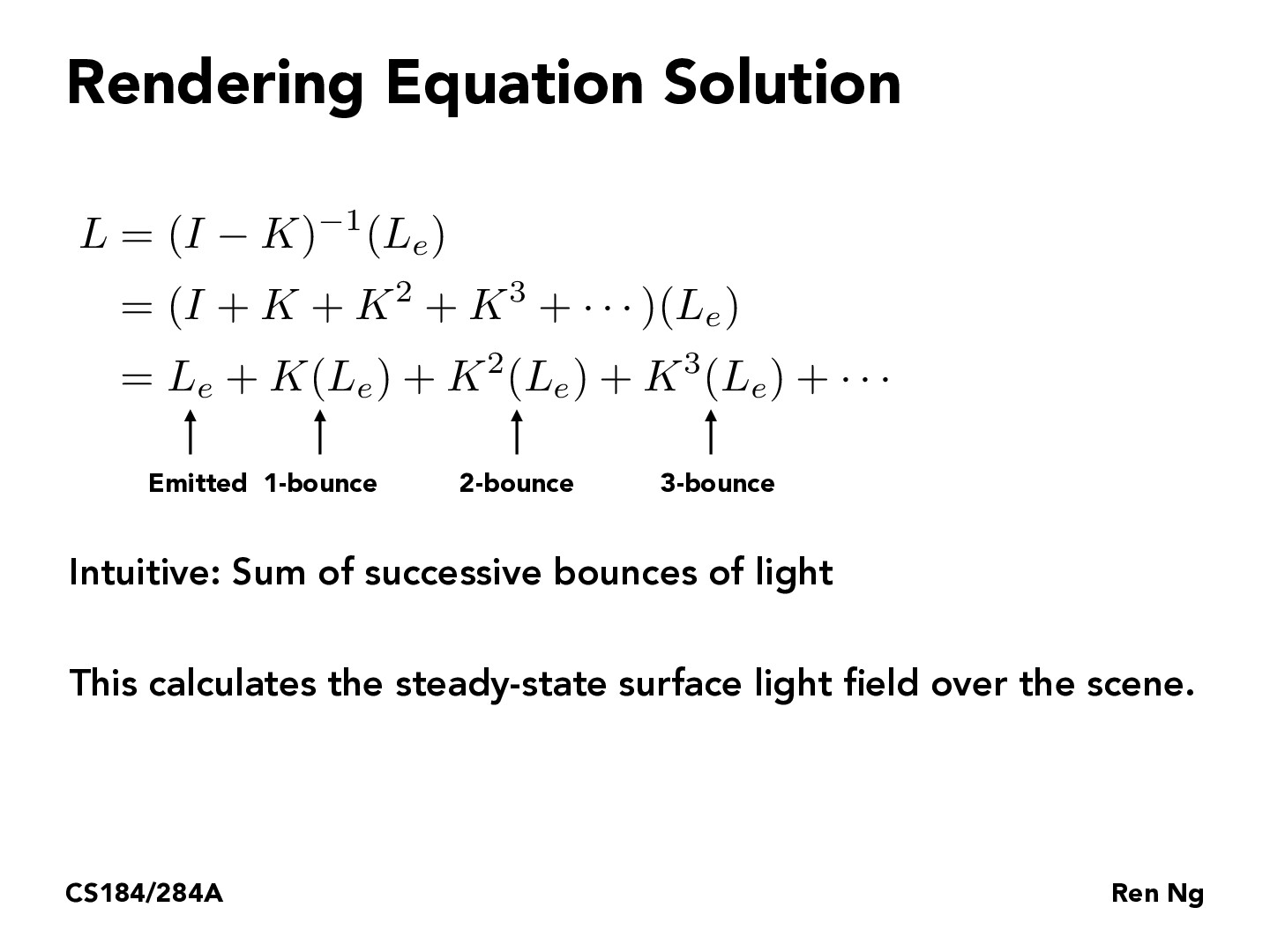
Breaking down rendering into the sum of successive bounces of light makes this equation a lot easier to understand and conceptualize. It's super interesting that the complex rendering equation can be simplified down into this. One thing I wonder is how many bounces do we need to go up to in order to create a realistic render. Does going to high result in overexposure, or make the rendering more accurate since in real life we don't place a limit on how many bounces of light there are between objects.
colinsteidtmann
@zyousafzai21, Based on later slides, I think the answer is that we stop when the scene "converges". I think this is when L stops changing as we add more bounces.
EDIT: actually it seems like we can terminate when we want using a fixed N, or with a strategy called "Russian Roulette" which is probabilistic termination. I wonder why we can't terminate when the light contributions converge?
SudhanvaKulkarni123
I wonder how K^n is computed for higher powers in practice. Is K diagonalizable? If so we can just use the Eigendecomposition to compute K^n for larger n. Else we need to pay an n^3 price for each power, which builds up very quickly! Since most things in nature tend to be "nice", I'm guessing it is indeed diagonalizable. If so, how do we prove it? If not, is there an efficient way to compute K^n for larger n? If my intuition is right, computing K^n will be even more expensive for environments with more geometric primitives due the large number of possible paths. It would make sense to pay a bit higher price at the start of the computation to find the Eigen values and vectors rather than just jumping into matrix multiply.
Breaking down rendering into the sum of successive bounces of light makes this equation a lot easier to understand and conceptualize. It's super interesting that the complex rendering equation can be simplified down into this. One thing I wonder is how many bounces do we need to go up to in order to create a realistic render. Does going to high result in overexposure, or make the rendering more accurate since in real life we don't place a limit on how many bounces of light there are between objects.
@zyousafzai21, Based on later slides, I think the answer is that we stop when the scene "converges". I think this is when L stops changing as we add more bounces.
EDIT: actually it seems like we can terminate when we want using a fixed N, or with a strategy called "Russian Roulette" which is probabilistic termination. I wonder why we can't terminate when the light contributions converge?
I wonder how K^n is computed for higher powers in practice. Is K diagonalizable? If so we can just use the Eigendecomposition to compute K^n for larger n. Else we need to pay an n^3 price for each power, which builds up very quickly! Since most things in nature tend to be "nice", I'm guessing it is indeed diagonalizable. If so, how do we prove it? If not, is there an efficient way to compute K^n for larger n? If my intuition is right, computing K^n will be even more expensive for environments with more geometric primitives due the large number of possible paths. It would make sense to pay a bit higher price at the start of the computation to find the Eigen values and vectors rather than just jumping into matrix multiply.