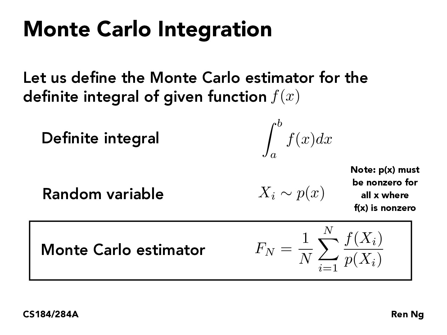
Note that in this definition, it doesn't matter how we define the pdf of X - it could even be uniform. The PDF is independent of the function values.
brandonlouie
In lecture, I believe it was mentioned that the Monte Carlo estimator was weighted. I'm interested to know why it's defined to be weighted by the inverse probability rather than the probability itself. I feel like the latter is more intuitive and akin to the formula for expected value. The only interpretation I have for the former is that we want to give less likely values more weight, but I'm not quite sure why. Did I miss something?
colinsteidtmann
Is the probability distribution discrete or continuous?
colinsteidtmann
@brandonlouie, I agree it's interesting that we divide instead of multiply. Note that probabilities have values less than 1, so this effectively makes the samples f(x) larger. Not sure if that helps us understand the division question any better.
saif-m17
@colinsteidtmann In response to your first question, I don't think there's a particular specification on whether the distribution is continuous or discrete, though both examples we've done have been with continuous distributions. My guess would be that there should be preference toward continuous distributions, since we're working with continuous functions (f), so we want to make sure that there exist density values for all x.
saif-m17
@brandonlouie/@colinsteidtmann In terms of why it makes sense to divide by p(x): it was mentioned that we wanted an unbiased estimator (i.e, the expectation of Fn should be equivalent to the integral we are estimating). When you take the expectation of Fn, you integrate and multiply this expression by p(x), so the p(x) terms cancel, resulting in just the integral value we want to estimate. So dividing allows us to ensure that the estimator is unbiased.
Mehvix
@brandonlouie Intuitively, if probability of some Xi is large then we will sample it often (it'd contribute to the sum proportional to p(Xi)). Diving by this probability ensures an unbiased estimator, i.e. each sample's contribution to the sum is weighted equally regardless of its probability
[edit] slide 40 gives another way to think about this:
"if I sample x less frequently, each sample should count more"
snowshoes7
@Mehvix wait, is that true? It looks to me like this would just be weighting by the inverse of the probability, no? Unless f(X) doesn't represent what I assumed it did.
Mehvix
@snowshoes7 Yes, that is what we are doing. f(Xi) is the fctn value corresponding to sample Xi. p(Xi) is the likelihood we pick sample Xi.
grafour
https://www.youtube.com/watch?v=WAf0rqwAvgg I was really confused initially looking at this, but there is a really good video giving examples as well so we can see how well this works.
s3kim2018
As Ren said in lecture, the probability of a point in the curve being selected is weighted by its probability. As N increases, the points that have a higher probability will have a smaller contribution as p(Xi) is larger. In subsequent examples, Ren used the Uniform RV to define a Monte Carlo estimator. Since the estimator weights the points by its relative probability, will we get the same result if we use any probability distribution with range (a~b)?
Edge7481
Ngl i should've tried harder to understand this part after getting destroyed in the exam
Note that in this definition, it doesn't matter how we define the pdf of X - it could even be uniform. The PDF is independent of the function values.
In lecture, I believe it was mentioned that the Monte Carlo estimator was weighted. I'm interested to know why it's defined to be weighted by the inverse probability rather than the probability itself. I feel like the latter is more intuitive and akin to the formula for expected value. The only interpretation I have for the former is that we want to give less likely values more weight, but I'm not quite sure why. Did I miss something?
Is the probability distribution discrete or continuous?
@brandonlouie, I agree it's interesting that we divide instead of multiply. Note that probabilities have values less than 1, so this effectively makes the samples f(x) larger. Not sure if that helps us understand the division question any better.
@colinsteidtmann In response to your first question, I don't think there's a particular specification on whether the distribution is continuous or discrete, though both examples we've done have been with continuous distributions. My guess would be that there should be preference toward continuous distributions, since we're working with continuous functions (f), so we want to make sure that there exist density values for all x.
@brandonlouie/@colinsteidtmann In terms of why it makes sense to divide by p(x): it was mentioned that we wanted an unbiased estimator (i.e, the expectation of Fn should be equivalent to the integral we are estimating). When you take the expectation of Fn, you integrate and multiply this expression by p(x), so the p(x) terms cancel, resulting in just the integral value we want to estimate. So dividing allows us to ensure that the estimator is unbiased.
@brandonlouie Intuitively, if probability of some Xi is large then we will sample it often (it'd contribute to the sum proportional to p(Xi)). Diving by this probability ensures an unbiased estimator, i.e. each sample's contribution to the sum is weighted equally regardless of its probability
[edit] slide 40 gives another way to think about this: "if I sample x less frequently, each sample should count more"
@Mehvix wait, is that true? It looks to me like this would just be weighting by the inverse of the probability, no? Unless f(X) doesn't represent what I assumed it did.
@snowshoes7 Yes, that is what we are doing. f(Xi) is the fctn value corresponding to sample Xi. p(Xi) is the likelihood we pick sample Xi.
https://www.youtube.com/watch?v=WAf0rqwAvgg I was really confused initially looking at this, but there is a really good video giving examples as well so we can see how well this works.
As Ren said in lecture, the probability of a point in the curve being selected is weighted by its probability. As N increases, the points that have a higher probability will have a smaller contribution as p(Xi) is larger. In subsequent examples, Ren used the Uniform RV to define a Monte Carlo estimator. Since the estimator weights the points by its relative probability, will we get the same result if we use any probability distribution with range (a~b)?
Ngl i should've tried harder to understand this part after getting destroyed in the exam