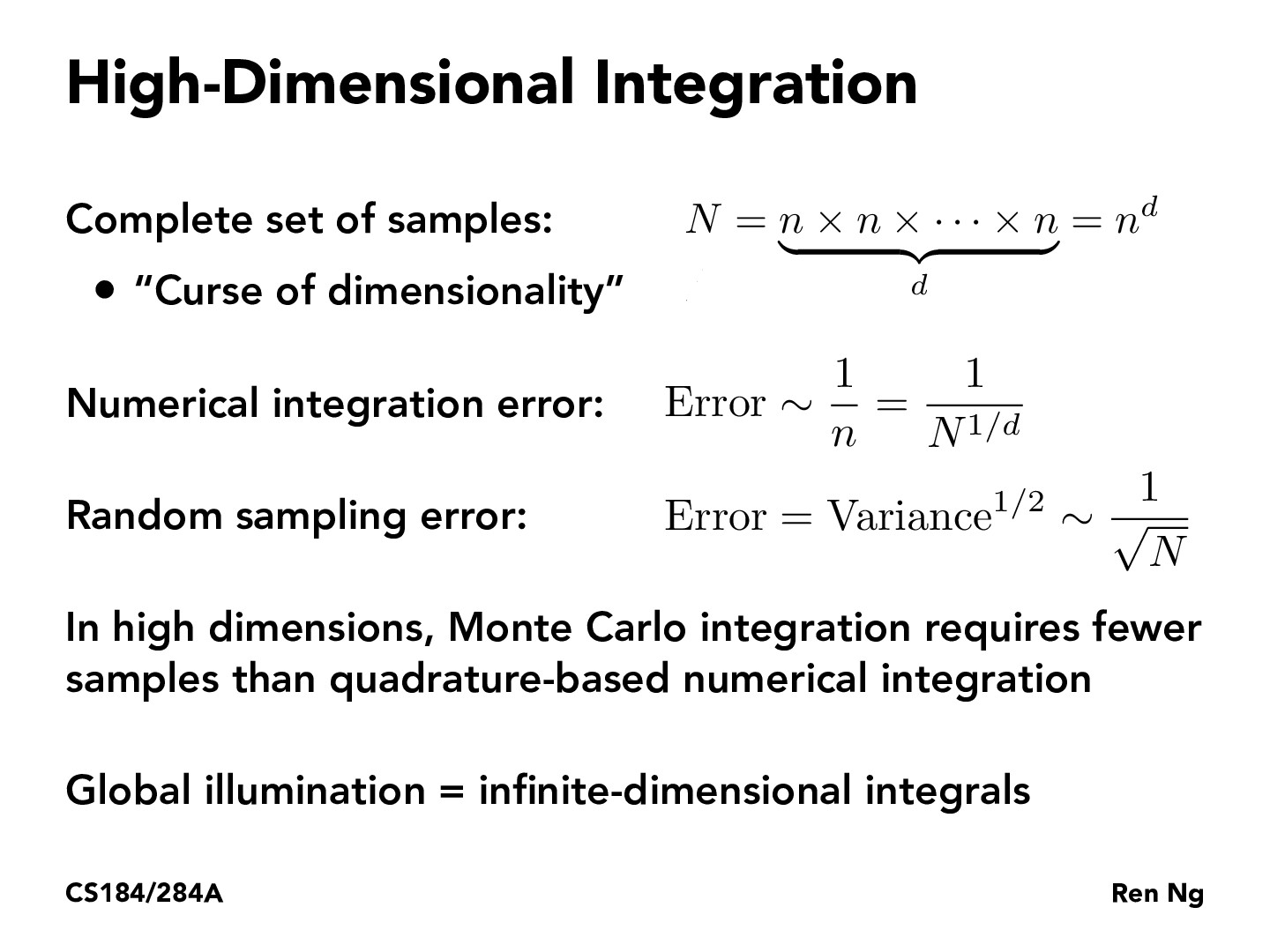
n here represents the number of samples at each dimension, and N represents the total number of samples taken
micahtyong
The "curse of dimensionality" shows up in places like rejection sampling, where we create a bounding box over our parameter space and accept samples with probabilities proportional to a target density function. In the 1D case, this works fine assuming we choose a tight bounding box and we get an acceptance rate of, say, 0.3. However, in the multi-dimensional setting, this acceptance rate tends to 0 as d increases (for reasons related to this slide).
A natural MCMC improvement to rejection sampling is Gibbs sampling, which essentially uses 1D rejection sampling as a subroutine to keep our acceptance rate moderately high.
n here represents the number of samples at each dimension, and N represents the total number of samples taken
The "curse of dimensionality" shows up in places like rejection sampling, where we create a bounding box over our parameter space and accept samples with probabilities proportional to a target density function. In the 1D case, this works fine assuming we choose a tight bounding box and we get an acceptance rate of, say, 0.3. However, in the multi-dimensional setting, this acceptance rate tends to 0 as d increases (for reasons related to this slide).
A natural MCMC improvement to rejection sampling is Gibbs sampling, which essentially uses 1D rejection sampling as a subroutine to keep our acceptance rate moderately high.